7 Analysis

7.1 srvyr package

“The srvyr package aims to add dplyr like syntax to the survey package.” It is a very useful package for a variety of aggregations of survey data.

###makes some additions. 
library(tidyverse)
library(srvyr)
library(kableExtra)
library(readxl)
df<-read_csv("inputs/UKR2007_MSNA20_HH_dataset_main_rcop.csv")

main_dataset <- read.csv("inputs/UKR2007_MSNA20_HH_dataset_main_rcop.csv", na.strings = "")
loop_dataset <- read.csv("inputs/UKR2007_MSNA20_HH_dataset_loop_rcop.csv", na.strings = "")

main_dataset <- main_dataset %>% select_if(~ !(all(is.na(.x)) | all(. == "")))

questions <- read_xlsx("inputs/UKR2007_MSNA20_HH_Questionnaire_24JUL2020.xlsx",sheet="survey")
choices <- read_xlsx("inputs/UKR2007_MSNA20_HH_Questionnaire_24JUL2020.xlsx",sheet="choices")
dfsvy<-as_survey(df)

7.1.1 Categorical variables

srvyr package allows categorical variables to be broken down using a similar syntax as dplyr. Using dplyr you might typically calculate a percent mean as follows:

df %>% 
  group_by(b9_hohh_marital_status) %>% 
  summarise(
    n=n()
  ) %>% 
  ungroup() %>% 
  mutate(
    pct_mean=n/sum(n)
  )

## # A tibble: 6 × 3
##   b9_hohh_marital_status                        n pct_mean
##   <chr>                                     <int>    <dbl>
## 1 divorced                                    183   0.113 
## 2 married                                     677   0.419 
## 3 separated_married_but_not_living_together    37   0.0229
## 4 single                                      129   0.0798
## 5 unmarried_but_living_together                96   0.0594
## 6 widowed                                     495   0.306

To calculate the percent mean of a categorical variable using srvyr object is required. The syntax is quite similar to dplyr, but a bit less verbose. By specifying the vartype as “ci” we also get the upper and lower confidence intervals

dfsvy %>% 
  group_by(b9_hohh_marital_status) %>% 
  summarise(
    pct_mean = survey_mean(vartype = "ci")
  )

## # A tibble: 6 × 4
##   b9_hohh_marital_status                    pct_mean pct_mean_low pct_mean_upp
##   <chr>                                        <dbl>        <dbl>        <dbl>
## 1 divorced                                    0.113        0.0977       0.129 
## 2 married                                     0.419        0.395        0.443 
## 3 separated_married_but_not_living_together   0.0229       0.0156       0.0302
## 4 single                                      0.0798       0.0666       0.0930
## 5 unmarried_but_living_together               0.0594       0.0478       0.0709
## 6 widowed                                     0.306        0.284        0.329

To calculate the weigthed percent mean of a multiple response option you need to created a srvyr object including the weights. The syntax is similar to dyplr and allows for the total columns

weighted_object <- main_dataset %>% as_survey_design(ids = X_uuid, weights = stratum.weight)

weighted_table <- weighted_object %>% 
                  group_by(adm1NameLat) %>% #group by categorical variable
                  summarise_at(vars(starts_with("b10_hohh_vulnerability.")), survey_mean) %>% #select multiple response question
                  ungroup() %>% 
                  bind_rows(
                            summarise_at(weighted_object,
                            vars(starts_with("b10_hohh_vulnerability.")), survey_mean) # bind the total
                  ) %>%
                mutate_at(vars(adm1NameLat), ~replace(., is.na(.), "Total")) %>% 
                select(., -(ends_with("_se"))) %>%  #remove the colums with the variance type calculations
                mutate_if(is.numeric, ~ . * 100) %>%
                mutate_if(is.numeric, round, 2)


print(weighted_table)

## # A tibble: 3 × 11
##   adm1NameLat b10_hohh_vulnerability.no b10_hohh_vulnerability… b10_hohh_vulner…
##   <chr>                           <dbl>                   <dbl>            <dbl>
## 1 Donetska                         30.0                    9.7              8.88
## 2 Luhanska                         15.2                    9.88             9.63
## 3 Total                            26.4                    9.74             9.07
## # … with 7 more variables: b10_hohh_vulnerability.veteran_of_war_ato <dbl>,
## #   b10_hohh_vulnerability.single_parent <dbl>,
## #   b10_hohh_vulnerability.family_with_3_or_more_children <dbl>,
## #   b10_hohh_vulnerability.family_with_foster_children <dbl>,
## #   b10_hohh_vulnerability.other_specify <dbl>,
## #   b10_hohh_vulnerability.chronic_illness <dbl>,
## #   b10_hohh_vulnerability.older_person <dbl>

7.1.2 Numeric variables

srvyr treats the calculation/aggregation of numeric variables differently in an attempt to mirror dplyr syntax

to calculate the mean and median expenditure in dplyr you would likely do the following

df %>% 
  summarise(
    mean_expenditure= mean(n1_HH_total_expenditure,na.rm=T),
    median_expenditure=median(n1_HH_total_expenditure,na.rm=T),
    )

## # A tibble: 1 × 2
##   mean_expenditure median_expenditure
##              <dbl>              <dbl>
## 1            5129.               4000

If you wanted to subset this by another variable in dplyr you would add the group_by argument

df %>% 
  group_by(strata) %>% 
  summarise(
    mean_expenditure= mean(n1_HH_total_expenditure,na.rm=T),
    median_expenditure=median(n1_HH_total_expenditure,na.rm=T),
    )

## # A tibble: 4 × 3
##   strata     mean_expenditure median_expenditure
##   <chr>                 <dbl>              <dbl>
## 1 20km_rural            5488.               4000
## 2 20km_urban            6208.               5000
## 3 5km_rural             3919.               3075
## 4 5km_urban             4942.               4000

This is the reason why the syntax also varies between categorical and numeric variables in srvyr. Therefore, to do the same using srvyr you would do the following (with a survey object). Note that due to this difference in syntax the na.rm argument works for numeric variables, but does not work for categorical variables. This was modified when srvyr was updated from v 0.3.8

dfsvy %>% 
  summarise(
   mean= survey_mean(n1_HH_total_expenditure,na.rm=T,vartype = "ci"),
  )

## # A tibble: 1 × 3
##    mean mean_low mean_upp
##   <dbl>    <dbl>    <dbl>
## 1 5129.    4891.    5367.

similar to dplyr you can easily add a group_by argument to add a subset calculation

dfsvy %>% 
  group_by(strata) %>% 
  summarise(
   mean= survey_mean(n1_HH_total_expenditure,na.rm=T,vartype = "ci"),
  )

## # A tibble: 4 × 4
##   strata      mean mean_low mean_upp
##   <chr>      <dbl>    <dbl>    <dbl>
## 1 20km_rural 5488.    4980.    5996.
## 2 20km_urban 6208.    5661.    6756.
## 3 5km_rural  3919.    3469.    4370.
## 4 5km_urban  4942.    4604.    5280.

7.1.3 select_one

7.1.4 select_mutiple

7.2 Analysis with numerical variables

7.2.1 Averages

###Summarytools (CRAN package)

###hypegrammaR / koboquest / butteR

7.2.2 Median

####Spatstat Spatstat - library with set of different functions for analyzing Spatial Point Patterns but also quite useful for analysis of weighted data.

At first let’s select all numerical variables from the dataset using Kobo questionnaire and dataset. It can be done with the following custom function:

library(spatstat)

## Loading required package: spatstat.data

## Loading required package: spatstat.geom

## spatstat.geom 3.0-3

## 
## Attaching package: 'spatstat.geom'

## The following object is masked from 'package:maditr':
## 
##     shift

## The following object is masked from 'package:grid':
## 
##     as.mask

## Loading required package: spatstat.random

## spatstat.random 3.0-1

## Loading required package: spatstat.explore

## Loading required package: nlme

## 
## Attaching package: 'nlme'

## The following object is masked from 'package:dplyr':
## 
##     collapse

## spatstat.explore 3.0-5

## Loading required package: spatstat.model

## Loading required package: rpart

## spatstat.model 3.0-2

## 
## Attaching package: 'spatstat.model'

## The following object is masked from 'package:expss':
## 
##     valid

## Loading required package: spatstat.linnet

## spatstat.linnet 3.0-3

## 
## spatstat 3.0-2 
## For an introduction to spatstat, type 'beginner'

select_numerical <- function(dataset, kobo){
  kobo_questions <- kobo[grepl("integer|decimal|calculate", kobo$type),c("type","name")]
  names.use <- names(dataset)[(names(dataset) %in% as.character(kobo_questions$name))]
  numerical <- dataset[,c(names.use,"X_uuid",'strata','stratum.weight')] #Here we can select any other relevant variables
  numerical[names.use] <- lapply(numerical[names.use], gsub, pattern = 'NA', replacement = NA)
  numerical[names.use] <- lapply(numerical[names.use], as.numeric)
  return(numerical)
}

numerical_questions <- select_numerical(main_dataset, questions)

numerical_classes <- sapply(numerical_questions[,1:c(ncol(numerical_questions)-3)], class) #Here we can check class of each selected variable
numerical_classes <- numerical_classes["character" %in% numerical_classes] #and here we check if any variable has class "character"
numerical_questions <- numerical_questions[ , !names(numerical_questions) %in% numerical_classes] #if any variable has a character class then we remove it
rm(numerical_classes)#and here we removing vector with classes from our environment

Now let’s calculate weighted median for “n1_HH_total_expenditure”.

weighted.median(numerical_questions$n1_HH_total_expenditure, numerical_questions$stratum.weight, na.rm=TRUE)

## [1] 4150

But if we want to calculate weighted medians for each variable we will need to iterate this function on those variables. But first we will need to exclude variables with less than 3 observations.

counts <- numerical_questions %>%
select(-X_uuid, -strata) %>%
summarise(across(.cols = everything(), .fns= ~sum(!is.na(.)) ))%>%
t()#Calculating count of observation for each variable

numerical_questions <- numerical_questions[ , (names(numerical_questions) %in% rownames(subset(counts, counts[,1] > 3)))]
#removing variables with less than 3 observations


medians <- lapply(numerical_questions[1:46], weighted.median, w = numerical_questions$stratum.weight, na.rm=TRUE)%>%
  as.data.frame()

Now we can transpond resulting vector and add description to the calculation

medians <- as.data.frame(t(medians),stringsAsFactors = FALSE)
names(medians)[1] <- "Median_wght"
head(medians)

##                               Median_wght
## b15_hohh_income                    2780.0
## hohh_age_18                           0.0
## age_18                                0.0
## b21_num_additional_hh_members         0.5
## age_5_18_number                       0.0
## age_5_12_number                       0.0

7.3 Ratios

This function computes the % of answers for select multiple questions.
The output can be used as a data merge file for indesign.
The arguments are: dataset, disaggregation variable, question to analyze, and weight column.

7.3.1 Example1:

Question: e11_items_do_not_have_per_hh
Disaggregation variable: b9_hohh_marital_status
weights column: stratum.weight

ratios_select_multiple <-
  function(df, x_var, y_prefix, weights_var) {
    df %>%
      group_by({
        {
          x_var
        }
      }) %>% filter(!is.na(y_prefix)) %>%
      summarize(across(starts_with(paste0(y_prefix, ".")),
                       list(pct = ~ weighted.mean(., {
                         {
                           weights_var
                         }
                       }, na.rm = T))))
  }

res <-
  ratios_select_multiple(
    main_dataset,
    b9_hohh_marital_status,
    "e11_items_do_not_have_per_hh",
    stratum.weight
  )

head(res)

## # A tibble: 6 × 5
##   b9_hohh_marital_status      e11_items_do_no… e11_items_do_no… e11_items_do_no…
##   <chr>                                  <dbl>            <dbl>            <dbl>
## 1 divorced                              0.0851           0.0859            0.393
## 2 married                               0.0496           0.0545            0.409
## 3 separated_married_but_not_…           0.0138           0.0513            0.443
## 4 single                                0.0726           0.0516            0.457
## 5 unmarried_but_living_toget…           0.0874           0.101             0.293
## 6 widowed                               0.106            0.0923            0.504
## # … with 1 more variable:
## #   e11_items_do_not_have_per_hh.hh_has_all_items_pct <dbl>

7.3.2 Example2 - Analyzing multiple questions and combine the output:

Question: e11_items_do_not_have_per_hh and b11_hohh_chronic_illness
Disaggregation variable: b9_hohh_marital_status
weights column: stratum.weight

res <-
  do.call("full_join", map(
    c("e11_items_do_not_have_per_hh", "b11_hohh_chronic_illness"),
    ~ ratios_select_multiple(main_dataset, b9_hohh_marital_status, .x, stratum.weight)
  ))

## Joining, by = "b9_hohh_marital_status"

head(res)

## # A tibble: 6 × 18
##   b9_hohh_marital_status      e11_items_do_no… e11_items_do_no… e11_items_do_no…
##   <chr>                                  <dbl>            <dbl>            <dbl>
## 1 divorced                              0.0851           0.0859            0.393
## 2 married                               0.0496           0.0545            0.409
## 3 separated_married_but_not_…           0.0138           0.0513            0.443
## 4 single                                0.0726           0.0516            0.457
## 5 unmarried_but_living_toget…           0.0874           0.101             0.293
## 6 widowed                               0.106            0.0923            0.504
## # … with 14 more variables:
## #   e11_items_do_not_have_per_hh.hh_has_all_items_pct <dbl>,
## #   b11_hohh_chronic_illness.blood_pressure_diseases_pct <dbl>,
## #   b11_hohh_chronic_illness.cardiovascular_disease_pct <dbl>,
## #   b11_hohh_chronic_illness.diabetes_need_insulin_pct <dbl>,
## #   b11_hohh_chronic_illness.diabetes_does_not_need_insulin_pct <dbl>,
## #   b11_hohh_chronic_illness.chronic_respiratory_condition_pct <dbl>, …

7.3.3 Example3 - No dissagregation is needed and/or the data is not weighted:

Question: e11_items_do_not_have_per_hh and b11_hohh_chronic_illness
Disaggregation variable: NA
weights column: NA

main_dataset$all <- "all"
main_dataset$no_weights <- 1

res <-
  do.call("full_join", map(
    c("e11_items_do_not_have_per_hh", "b11_hohh_chronic_illness"),
    ~ ratios_select_multiple(main_dataset, all, .x, no_weights)
  ))

## Joining, by = "all"

head(res)

## # A tibble: 1 × 18
##   all   e11_items_do_not_hav… e11_items_do_no… e11_items_do_no… e11_items_do_no…
##   <chr>                 <dbl>            <dbl>            <dbl>            <dbl>
## 1 all                  0.0804           0.0779            0.417            0.515
## # … with 13 more variables:
## #   b11_hohh_chronic_illness.blood_pressure_diseases_pct <dbl>,
## #   b11_hohh_chronic_illness.cardiovascular_disease_pct <dbl>,
## #   b11_hohh_chronic_illness.diabetes_need_insulin_pct <dbl>,
## #   b11_hohh_chronic_illness.diabetes_does_not_need_insulin_pct <dbl>,
## #   b11_hohh_chronic_illness.chronic_respiratory_condition_pct <dbl>,
## #   b11_hohh_chronic_illness.musculoskeletal_system_and_joints_pct <dbl>, …

7.4 Weights

Weights can be used for different reasons. In most of cases, we will use weights to correct for difference between strata size. Once the population has a certain (big) size, for the same design, the size of the sample won’t change much. In the case of the dataset, there are 4 stratas:
- within 20km of the border in rural areas : 89,408 households
- within 20km of the border in urban areas : 203,712 households
- within 20km of the border in rural areas : 39,003 households
- within 20km of the border in rural areas : 211,857 households

Using any sampling calculator, for a 95% confindence level, 5% margin of error and 5% buffer, we will have around 400 samples per strata even though the urban areas are much bigger.
Note: The error of 5% for 90,000 is 4,500 households while for 200,000 households is 10,000 households

If we look at each strata and the highest level of education completed by the household head (b20_hohh_level_education), we can see that the percentage of household were the head of household completed higher education varies between between 7 to 13 % in each strata.

## # A tibble: 4 × 5
## # Groups:   strata [4]
##   strata     b20_hohh_level_education     n tot_n  prop
##   <chr>      <chr>                    <int> <int> <dbl>
## 1 20km_rural complete_higher             40   407    10
## 2 20km_urban complete_higher             51   404    13
## 3 5km_rural  complete_higher             38   402     9
## 4 5km_urban  complete_higher             28   404     7

However, if we want to know overall the percentage of who finished higher education we cannot just take the overall percentages, i.e. \(\frac{40 + 51 +38 + 28}{407 + 404 + 402 + 404}\) = \(\frac{157}{1617}\) = 10%.
We cannot do this because the first strata represent 90,000 households, the second 200,000 households, the third 40,000 households and the last one 210,000 households. We will use weights to compensate this difference.

We will use this formula:
weight of strata = \(\frac{\frac{strata\\ population}{total\\ population}}{\frac{strata\\ sample}{total\\ sample}}\)

7.4.1 tidyverse

The following example will show how to calculate the weights with tidyverse.

To calculate weights, we will need all the following information: - population of the strata,
- total population,
- sample and
- total sample.
The population information should come from the sampling frame that was used to draw the sampling.

my_sampling_frame <- readxl::read_excel("inputs/UKR2007_MSNA20_GCA_Weights_26AUG2020.xlsx", 
                                        sheet = "for_r") %>% 
  rename(population_strata = population)
my_sampling_frame

## # A tibble: 4 × 2
##   strata     population_strata
##   <chr>                  <dbl>
## 1 20km_rural             89408
## 2 20km_urban            230712
## 3 5km_rural              39003
## 4 5km_urban             211857

Then, we need to get the actual sample from the dataset.

sample_per_strata_table <- main_dataset %>% 
  group_by(strata) %>% 
  tally() %>% 
  rename(strata_sample = n) %>% 
  ungroup()

sample_per_strata_table

## # A tibble: 4 × 2
##   strata     strata_sample
##   <chr>              <int>
## 1 20km_rural           407
## 2 20km_urban           404
## 3 5km_rural            402
## 4 5km_urban            404

Then, we can join the tables together and calculate the weights per strata.

weight_table <- sample_per_strata_table %>% 
  left_join(my_sampling_frame) %>% 
  mutate(weights = (population_strata/sum(population_strata))/(strata_sample/sum(strata_sample)))

weight_table

## # A tibble: 4 × 4
##   strata     strata_sample population_strata weights
##   <chr>              <int>             <dbl>   <dbl>
## 1 20km_rural           407             89408   0.622
## 2 20km_urban           404            230712   1.62 
## 3 5km_rural            402             39003   0.275
## 4 5km_urban            404            211857   1.49

Then we can finally add them to the dataset.

main_dataset <- main_dataset %>% 
  left_join(select(weight_table, strata, weights), by = "strata")
head(main_dataset$weights)

## [1] 0.2747648 0.2747648 0.6221156 0.6221156 0.6221156 0.6221156

We can check that each strata has only 1 weight.

main_dataset %>% 
  group_by(strata, weights) %>%
  tally()

## # A tibble: 4 × 3
## # Groups:   strata [4]
##   strata     weights     n
##   <chr>        <dbl> <int>
## 1 20km_rural   0.622   407
## 2 20km_urban   1.62    404
## 3 5km_rural    0.275   402
## 4 5km_urban    1.49    404

We can check that the sum of weights is equal to the number of interviews.

sum(main_dataset$weights) == nrow(main_dataset)

## [1] TRUE

7.4.2 surveyweights

surveyweights was created to calculate weights. The function weighting_fun_from_samplingframe creates a function that calculates weights from the dataset and the sampling frame.

Note: surveyweights can be found on github.

First you need to create the weighting function. weighting_fun_from_samplingframe will take 5 arguments:
- sampling.frame: a data frame with your population figures and stratas.
- data.stratum.column : column name of the strata in the dataset.
- sampling.frame.population.column : column name of population figures in the sampling frame.
- sampling.frame.stratum.column : column name of the strata in the sampling frame.
- data : dataset

library(surveyweights)

## 
## Attaching package: 'surveyweights'

## The following object is masked from 'package:hypegrammaR':
## 
##     combine_weighting_functions

my_weigthing_function <- surveyweights::weighting_fun_from_samplingframe(sampling.frame = my_sampling_frame,
                                                                      data.stratum.column = "strata",
                                                                      sampling.frame.population.column = "population_strata", 
                                                                      sampling.frame.stratum.column = "strata", 
                                                                      data = main_dataset)

See that the my_weigthing_function is not a vector of weights. It is a function that takes the dataset as argument and returns a vector of weights.

is.function(my_weigthing_function)

## [1] TRUE

my_weigthing_function

## function (df) 
## {
##     if (!is.data.frame(df)) {
##         stop("df must be a data.frame")
##     }
##     df <- as.data.frame(df, stringsAsFactors = FALSE)
##     df <- lapply(df, function(x) {
##         if (is.factor(x)) {
##             return(as.character(x))
##         }
##         x
##     }) %>% as.data.frame(stringsAsFactors = FALSE)
##     if (!all(data.stratum.column %in% names(df))) {
##         stop(paste0("data frame column '", data.stratum.column, 
##             "'not found."))
##     }
##     df[[data.stratum.column]] <- as.character(df[[data.stratum.column]])
##     sample.counts <- stratify.count.sample(data.strata = asdhk[[data.stratum.column]], 
##         sf.strata = population.counts)
##     if ("weights" %in% names(df)) {
##         warning("'weights' is used as a column name (will not be calculated from the sampling frame)")
##     }
##     if (!all(names(sample.counts) %in% names(population.counts))) {
##         stop("all strata names in column '", data.stratum.column, 
##             "' must also appear in the loaded sampling frame.")
##     }
##     weights <- stratify.weights(pop_strata = population.counts, 
##         sample_strata = sample.counts)
##     return(weights[df[[data.stratum.column]]])
## }
## <bytecode: 0x0000026b70132418>
## <environment: 0x0000026b70108cd8>

my_weigthing_function(main_dataset) %>% head()

## Warning in my_weigthing_function(main_dataset): 'weights' is used as a column
## name (will not be calculated from the sampling frame)

## data.strata
##  5km_rural  5km_rural 20km_rural 20km_rural 20km_rural 20km_rural 
##  0.2747648  0.2747648  0.6221156  0.6221156  0.6221156  0.6221156

Note: A warning shows that if the column weights exists in the dataset, my_weigthing_function will not calculate weights. We need to remove the weights column from the previous example.

main_dataset$weights <- NULL
my_weigthing_function(main_dataset) %>% head()

## data.strata
##  5km_rural  5km_rural 20km_rural 20km_rural 20km_rural 20km_rural 
##  0.2747648  0.2747648  0.6221156  0.6221156  0.6221156  0.6221156

To add the weights, we need to add a new column.

main_dataset$my_weights <- my_weigthing_function(main_dataset)

head(main_dataset$my_weights)

## [1] 0.2747648 0.2747648 0.6221156 0.6221156 0.6221156 0.6221156

As for the previous example, we can check that only 1 weight is used per strata.

main_dataset %>% 
  group_by(strata, my_weights) %>% 
  tally()

## # A tibble: 4 × 3
## # Groups:   strata [4]
##   strata     my_weights      n
##   <chr>      <table[1d]> <int>
## 1 20km_rural 0.6221156     407
## 2 20km_urban 1.6172529     404
## 3 5km_rural  0.2747648     402
## 4 5km_urban  1.4850825     404

We can check that the sum of weights is equal to the number of interviews.

sum(main_dataset$my_weights) == nrow(main_dataset)

## [1] TRUE

7.5 impactR, based on `srvyr`

impactR was at first designed for helping data officers to cover most of the research cycles’ parts, from producing cleaning log, cleaning data, and analyzing it. It is available for download here: https://gnoblet.github.io/impactR/.

The visualization (post-analysis) component has now been moved to package visualizeR: https://gnoblet.github.io/visualizeR/. Composite indicators now lies into humind : https://github.com/gnoblet/humind. Analysis is still a module of impactR; yet it will most probably shortly be moved to a smaller consolidated packages.

There are some vignettes/some documentation on the Github website. In particular this one for analysis: https://gnoblet.github.io/impactR/articles/analysis.html.

You can install and load it with:

# devtools::install_github("gnoblet/impactR")
library(impactR)

## 
## Attaching package: 'impactR'

## The following objects are masked _by_ '.GlobalEnv':
## 
##     choices, cleaning_log

7.5.1 Introduction

7.5.1.1 Caveats

Though it has been used for several research cycles, including MSNAs, there is no test designed in the package. One discrepancy will be corrected in the next version using function make_analysis_from_dap(): it for now assumes that all id_analysis are distinct and not NAs when using bind = TRUE. The next version will also have a new feature: unweighted counts and some automation for select one and select multiple questions.

Grouping is for now only possible for one variable. If you want to disagregate for instance by setting (rural vs. urban) and admin1, then you must mutate a new variable beforehand (it is as simple as pasting both columns).

7.5.1.2 Rational

The package is a wrapper around srvyr. The workflow is as follows:

Prepare data: Get your data, weights, strata ready, and prepare a survey design object (using srvyr::as_survey_design()).
Individual general analysis: It has a small family of functions svy_*() such as svy_prop() which are wrappers around the srvyr::survey_*() family in order to harmonize outputs. These functions can be used on their owns and covers mean, median, ration, proportion, interaction.
Individual analysis based on a Kobo tool: Prepare your Kobo tool, then use make_analysis().
Multiple analyses based on a Kobo tool: Prepare your Data Analysis Plan, then feed make_analysis_from_dap().

7.5.1.3 Prepare data

Data must have been imported with ìmport_xlsx() or import_csv() or with janitor::clean_names(). This is to ensure that column names for multiple choices follow this pattern: “variable_choice1”, with an underscore between the variable name from the survey sheet and the choices from the choices sheet. For instance, for the main drinking water source (if multiple choice), it could be “w_water_source_surface_water” or “w_water_source_stand_pipe”.

7.5.2 First stage: prepare data and survey design

We start by downloading a dataset and the associated Kobo tool.

# The dataset (main and roster sheets), and the Kobo tool sheets are saved as a RDS object
all <- readRDS("inputs/REACH_HTI_dataset_MSNA-2022.RDS")

# Sheet main contains the HH data
main <- all$main

# Sheet survey contains the survey sheet
survey <- all$survey

# Sheet choices contains, well, the choices sheet
choices <- all$choices

Let’s prepare:

data with janitor::clean_names() to ensure lower case and only underscore (no dots, no /, etc.).
survey and choices: let’s separate column type from survey and rename the label column we want to keep to label, otherwise most functions won’t work.

main <- main |> 
  # To get clean_names()
  janitor::clean_names() |> 
  # To get better types
  readr::type_convert()

## 
## ── Column specification ─────────────────────────────────────
## cols(
##   .default = col_character()
## )
## ℹ Use `spec()` for the full column specifications.

survey <- survey |> 
  # To get clean names
  janitor::clean_names() |> 
  # To get two columns one for the variable type, and one for the list_name
  impactR::split_survey(type) |> 
  # To get one column labelled "label" if multiple languages are used
  dplyr::rename(label = label_francais)

choices <- choices |> 
  janitor::clean_names() |> 
  dplyr::rename(label = label_francais)

Now that the dataset and the Kobo tool are loaded, we can prepare the survey design:

design <- main |> 
  srvyr::as_survey_design(
    strata = stratum,
    weights = weights)

7.5.3 Second stage: One variable analysis

Let’s give a few examples for the svy_*() family.

# Median of respondent's age, with the confidence interval, no grouped analysis
impactR::svy_median(design, i_enquete_age, vartype = "ci")

## # A tibble: 1 × 3
##   median median_low median_upp
##    <dbl>      <dbl>      <dbl>
## 1     42         42         43

# Proportion of respondent's gender, with the confidence interval, by setting (rural vs. urban)
impactR::svy_prop(design, i_enquete_genre, milieu, vartype = "ci")

## # A tibble: 4 × 5
##   milieu i_enquete_genre  prop prop_low prop_upp
##   <chr>  <chr>           <dbl>    <dbl>    <dbl>
## 1 rural  femme           0.598    0.570    0.626
## 2 rural  homme           0.402    0.374    0.430
## 3 urbain femme           0.595    0.573    0.616
## 4 urbain homme           0.405    0.384    0.427

# Ratio of the number of 0-17 yo children that attended school, with the confidence interval and no group
impactR::svy_ratio(design, e_formellet, c_total_age_3a_17a, vartype = "ci")

## # A tibble: 1 × 3
##   ratio ratio_low ratio_upp
##   <dbl>     <dbl>     <dbl>
## 1 0.864     0.853     0.875

# Top 6 common profiles between type of sanitation and source of drinking water, by setting
impactR::svy_interact(design, c(h_2_type_latrine, h_1_principal_source_eau), group = milieu, vartype = "ci") |> head(6)

## # A tibble: 6 × 6
##   milieu h_2_type_latrine     h_1_principal_source_eau   prop prop_low prop_upp
##   <chr>  <chr>                <chr>                     <dbl>    <dbl>    <dbl>
## 1 rural  trou_ouvert          source_non_protege       0.122    0.104    0.140 
## 2 rural  defecation_air_libre source_non_protege       0.118    0.100    0.137 
## 3 rural  trou_ouvert          robinet_public           0.0707   0.0564   0.0851
## 4 urbain toilette_chasse_eau  reseau_dinepa            0.0679   0.0588   0.0770
## 5 urbain trou_ouvert          robinet_public           0.0664   0.0543   0.0784
## 6 urbain toilette_chasse_eau  camion_citerne           0.0526   0.0445   0.0607

## It means that unprotected water springs and open pit is the most common profile for rural hhs (12%), whereas the most common profile for urban hhs is flush and pour toilet and tap water with national network (7%).

7.5.4 Third stage: one analysis at a time with the Kobo tool

Now that we understands the svy_*() family of functions, we can use make_analysis() which is a wrapper around those for making analysis for medians, means, ratios, proportions of select ones and select multiples. The output of make_analysis() has standardized columns among all types of analysis and labels are pulled out if possible thanks to the survey and choices sheets.

Let’s say you don’t have a full DAP sheet, and you just want to make individual analyses.

1- Proportion for a single choice question:

# Single choice question, sanitation facility type
impactR::make_analysis(design, survey, choices, h_2_type_latrine, "prop_simple", level = 0.95, vartype = "ci")

# Same thing without labels, do not get labels of choices
impactR::make_analysis(design, survey, choices, h_2_type_latrine, "prop_simple", get_label = FALSE)

# Single choice question, by group setting (rural vs. urban) - group needs to be a character string here
impactR::make_analysis(design, survey, choices, h_2_type_latrine, "prop_simple", group = "milieu")

2- Proportion overall: calculate the proportion with NAs as a category, this can be useful in case of a skip logic and you want to make the calculation over the whole population:

# Single choice question: 
impactR::make_analysis(design, survey, choices, r_1_date_reception_assistance, "prop_simple_overall", none_label = "No assistance received, do not know, prefere not to say, or missing data")

3- Multiple proportion:

# Multiple choice question, here computing self-reported priority needs
impactR::make_analysis(design, survey, choices, r_1_besoin_prioritaire, "prop_multiple", level = 0.95, vartype = "ci")

# Multiple choice question, with no label and with groups
impactR::make_analysis(design, survey, choices, r_1_besoin_prioritaire, "prop_multiple", get_label = FALSE, group = "milieu")

4- Multiple proportion overall: calculate the proportion for each choice over the whole population (replaces NAs by 0s in the dummy columns):

# Multiple choice question, estimates calculated over the whole population.
impactR::make_analysis(design, survey, choices, r_1_besoin_prioritaire, "prop_multiple_overall")

5- Mean, median and counting numeric as character:

# Mean of interviewee's age
impactR::make_analysis(design, survey, choices, i_enquete_age, "mean")

# Median of interviewee's age
impactR::make_analysis(design, survey, choices, i_enquete_age, "median")

# Proportion counting a numeric variable as a character variable
# Could be used for some particular numeric variables. For instance, below is the % of HHs by daily duration of access to electricity by setting (rural or urban).
impactR::make_analysis(design, survey, choices, a_6_acces_courant, "count_numeric", group = "milieu")

6 - Last but not least, ratios (it does not consider NAs). For this, it is only necessary to write a character string with the two variable names separated by a comma:

# Let's calculate the % of children aged 3-17 that were registered to a formal school among the HHs that reported having children aged 3-17.
impactR::make_analysis(design, survey, choices, "e_formellet,c_total_age_3a_17a", "ratio")

7.5.4.1 Fourth stage: Using a data analysis plan

Now we can use a dap, which mainly consists of a data frame with needed information for performing the analysis. One line is one requested analysis. All variables in the dap must exist in the dataset to be analysed. Usually an excel sheet is the easiest way to go as it can be co-constructed by both an AO and a DO.

# Here I produce a three-line DAP directly in R just for the sake of the example.
dap <- tibble::tibble(
  # Column: unique analaysis id identifier
  id_analysis = c("foodsec_1", "foodsec_3", "foodsec_3"),
  # Column: sector/research question
  rq = c("FSL", "FSL", "FSL"),
  # Column: sub-sector, sub research question
  sub_rq = c("Food security", "Food security", "Livelihoods"),
  # Column: indicator name
  indicator = c("% of HHs by FCS category", "% of HHs by HHS level", "% of HHs by LCSI category"),
  # Column: recall period
  recall = c("7 days", "30 days", "30 days"),
  # Column: the variable name in the dataset 
  question_name = c("fcs_cat", "hhs_cat", "lcs_cat"),
  # Column: subset (to be written by hand, does the calculation operates on a substed of the population)
  subset = c(NA_character_, NA_character_, NA_character_),
  # Column: analysis name to be passed to `make_analysis()`
  analysis = c("prop_simple", "prop_simple", "prop_simple"),
  # Column: analysis name used to be displayed later on
  analysis_name = c("Proportion", "Proportion", "Proportion"),
  # Column: if using analysis "prop_simple_overall", what is the label for NAs, passed through `make_analysis()`
  none_label = c(NA_character_, NA_character_, NA_character_),
  # Column: group label
  group_name = "General population",
  # Column: group variable from which to disaggregate (setting as an example)
  group = c("milieu", "milieu", "milieu"),
  # Column: level of confidence
  level = c(0.95, 0.95, 0.95),
  # Column: should NAs be removed?
  na_rm = c("TRUE", "TRUE", "TRUE"),
  # Column! var type, here we want confidence intervals
  vartype = c("ci", "ci", "ci")
)

dap

## # A tibble: 3 × 15
##   id_analysis rq    sub_rq        indicator recall question_name subset analysis
##   <chr>       <chr> <chr>         <chr>     <chr>  <chr>         <chr>  <chr>   
## 1 foodsec_1   FSL   Food security % of HHs… 7 days fcs_cat       <NA>   prop_si…
## 2 foodsec_3   FSL   Food security % of HHs… 30 da… hhs_cat       <NA>   prop_si…
## 3 foodsec_3   FSL   Livelihoods   % of HHs… 30 da… lcs_cat       <NA>   prop_si…
## # … with 7 more variables: analysis_name <chr>, none_label <chr>,
## #   group_name <chr>, group <chr>, level <dbl>, na_rm <chr>, vartype <chr>

Let’s produce an analysis:

# Getting a list
an <- impactR::make_analysis_from_dap(design, survey, choices, dap)
# Note that if the variables' labels cannot be found in the Kobo tool, the variable's values are used as choices labels

# Getting a long dataframe
impactR::make_analysis_from_dap(design, survey, choices, dap, bind = TRUE) |> head(10)

# To perform the same analysis without grouping, you can just replace the "group" variable by NAs
dap |> 
  srvyr::mutate(group = rep(NA_character_, 3)) |> 
  impactR::make_analysis_from_dap(design, survey, choices, dap = _, bind = TRUE) |> 
  head(10)

7.6 EXAMPLE :: Survey analysis using illuminate

illuminate is designed for making the data analysis easy and less time consuming. The package is based on tidyr, dplyr,srvyr packages.You can install the package from here. HOWEVER the package is not maintained by the author anymore and it doesnt includes any tests.

7.6.1 Step 0:: Call libraries

library(illuminate)
library(tidyverse)
library(purrr)
library(readxl)
library(openxlsx)
library(srvyr)

7.6.2 Step 1:: Read data

Read data with read_sheets(). This will make sure your data is stored as appropriate data type. It is important to make sure that all the select multiple are stored as logical, otherwise un weighted count will be wrong. It is recommended to use the read_sheets() to read the data. use `?read_sheets() for more details.

#  [recommended] read_sheets("[datapath]",data_type_fix = T,remove_all_NA_col = T,na_strings = c("NA",""," "))
data_up<-read.csv("inputs/UKR2007_MSNA20_HH_dataset_main_rcop.csv")

The above code will give a dataframe called data_up

7.6.3 Step OPTIONAL:: Preaparing the data

ONLY APPLICABLE WHEN YOU ARE NOT READING YOUR DATA WITH read_sheets()

# data_up <- read_excel("data/data.xlsx")
data_up <- fix_data_type(df = data_up)

7.6.4 Step 2:: Weight calculation

To do the weighted analysis, you will need to calculate the weights. If your dataset already have the weights column then you can ignore this part

7.6.5 Read sampleframe

# dummy code.
sampling_frame <- read.csv("[Sample frame path]")

This will give a data frame called sampling_frame

# dummy code.

weights <- data_up %>% group_by(governorate1) %>% summarise(
  survey_count = n()
) %>% left_join(sampling_frame,by =c("governorate1"="strata.names")) %>% 
  mutate(sample_global=sum(survey_count),
         pop_global=sum(population),
         survey_weight= (population/pop_global)/(survey_count/sample_global)) %>% select(governorate1,survey_weight)

7.6.6 Add weights to the dataframe

# dummy code.
data_up <- data_up %>% left_join(weights,by= "governorate1")

7.6.7 Step 3.1:: Weighted analysis

To do the weighted analysis, you need to set weights parameter to TRUE and provide weight_column and strata. You should define the name of the data set weight column in the weight_column parameter and name of the strata column name from the data set.

Additionally, please define the name of the columns which you would like to analyze in vars_to_analyze. Default will analyze all the variables that exist in the data set.

Lastly, please define the sm_sep parameter carefully. It must be either / or ,. Use / when your select multiple type questions are separated by / (example- parent_name/child_name1,parent_name/child_name2, parent_name/child_name3…..). On the other hand use . when the multiple choices are separated by .. (example - parent_name.child_name1,parent_name.child_name2,parent_name.child_name3)

# dummy code.

overall_analysis <- survey_analysis(df = data_up,weights = T,weight_column = "survey_weight",strata = "governorate1")

# As var_to_analyze is not defined, here the function will analyze all the variables.

7.6.8 Step 3.2:: Unweighted analysis

To do unweighted analysis, you need to set the weights parameter FALSE.

columns_to_analyze <- data_up[20:50] %>% names() ## Defining  names of the variables to be analyzed. 
overall_analysis <- survey_analysis(df = data_up,weights = F,vars_to_analyze = columns_to_analyze )

## [1] "b10_1_hohh_vulnerability_other"
## [1] "b11_hohh_chronic_illness.blood_pressure_diseases"
## [1] "b11_hohh_chronic_illness.cardiovascular_disease"
## [1] "b11_hohh_chronic_illness.diabetes_need_insulin"
## [1] "b11_hohh_chronic_illness.diabetes_does_not_need_insulin"
## [1] "b11_hohh_chronic_illness.chronic_respiratory_condition"
## [1] "b11_hohh_chronic_illness.musculoskeletal_system_and_joints"
## [1] "b11_hohh_chronic_illness.cancer"
## [1] "b11_hohh_chronic_illness.neurological"
## [1] "b11_hohh_chronic_illness.sensory_disorder"
## [1] "b11_hohh_chronic_illness.gastrointestinal_digestive_tract_incl_liver_gallbladder_pancreas_diseases"
## [1] "b11_hohh_chronic_illness.genitourinary_system_diseases"
## [1] "b11_hohh_chronic_illness.endocrine_system_thyroid_gland_and_other_diseases"
## [1] "b11_hohh_chronic_illness.other_specify"
## [1] "b11_1_hohh_chronic_illness_other"
## [1] "b12_situation_description"
## [1] "b12_1_situation_description_other"
## [1] "b13_why_hohh_unemployed"
## [1] "b13_1_why_hohh_unemployed_other"
## [1] "b14_sector_hohh_employed"
## [1] "b14_1_sector_hohh_employed_other"
## [1] "b15_hohh_income"
## [1] "b16_hohh_pension_eligible"
## [1] "b17_hohh_pension_receive"
## [1] "b18_hohh_benefit_eligible"
## [1] "b19_hohh_benefit_receive"
## [1] "b20_hohh_level_education"
## [1] "hohh_age_18"
## [1] "age_18"
## [1] "b21_num_additional_hh_members"
## [1] "b11_hohh_chronic_illness.blood_pressure_diseases"
## [1] "b11_hohh_chronic_illness.cardiovascular_disease"
## [1] "b11_hohh_chronic_illness.diabetes_need_insulin"
## [1] "b11_hohh_chronic_illness.diabetes_does_not_need_insulin"
## [1] "b11_hohh_chronic_illness.chronic_respiratory_condition"
## [1] "b11_hohh_chronic_illness.musculoskeletal_system_and_joints"
## [1] "b11_hohh_chronic_illness.cancer"
## [1] "b11_hohh_chronic_illness.neurological"
## [1] "b11_hohh_chronic_illness.sensory_disorder"
## [1] "b11_hohh_chronic_illness.gastrointestinal_digestive_tract_incl_liver_gallbladder_pancreas_diseases"
## [1] "b11_hohh_chronic_illness.genitourinary_system_diseases"
## [1] "b11_hohh_chronic_illness.endocrine_system_thyroid_gland_and_other_diseases"
## [1] "b11_hohh_chronic_illness.other_specify"

DT::datatable(overall_analysis,caption = "Example::Analysis table")

7.6.9 Step 3.3:: Weighted and disaggregated by gender analysis

Use ?survey_analysis() to know about the perameters.

# dummy code.
analysis_by_gender <-  survey_analysis(df = data_up,weights = T,weight_column = "survey_weight",vars_to_analyze = columns_to_analyze,
                                       strata = "governorate1",disag = c("va_child_income","gender_speaker"))

7.6.10 Step 4:: Export with `write_formatted_excel()`

You can use any function to export the analysis however write_formatted_excel() can export formatted file. See the documentation for more details.

write_list <- list(overall_analysis ="overall_analysis",
                   analysis_by_gender ="analysis_by_gender"
)
write_formatted_excel(write_list,"analysis_output.xlsx",
                      header_front_size = 12,
                      body_front = "Times")

7.7 Repeating the above

7.8 Analysis - top X / ranking (select one and select multiple)

First: select_one question

The indicator of interest is e1_shelter_type and the options are:

solid_finished_house
solid_finished_apartment
unfinished_nonenclosed_building
collective_shelter
tent
makeshift_shelter
none_sleeping_in_open
other_specify
dont_know_refuse_to_answer

# Top X/ranking for select_one type questions 
select_one_topX <- function(df, question_name, X=3, weights_col=NULL, disaggregation_col=NULL){
  # test message
  if(length(colnames(df)[grepl(question_name, colnames(df), fixed = T)]) == 0) {
    stop(print(paste("question name:", question_name, "doesn't exist in the main dataset. Please double check and make required changes!")))
  }
  
  #### no disag
  if(is.null(disaggregation_col)){
    #no weights 
    if(is.null(weights_col)){
    df <- df %>% 
      filter(!is.na(!!sym(question_name))) %>%
      group_by(!!sym(question_name)) %>%
      summarize(n=n()) %>%
      mutate(percentages = round(n / sum(n) * 100, digits = 2)) %>%
      select(!!sym(question_name), n, percentages) %>%
      arrange(desc(percentages)) %>% 
      head(X)
    }

    # weights 
    if(!is.null(weights_col)){
    df <- df %>% 
      filter(!is.na(!!sym(question_name))) %>%
      group_by(!!sym(question_name)) %>%
      summarize(n=sum(!!sym(weights_col))) %>%
      mutate(percentages = round(n / sum(n) * 100, digits = 2)) %>%
      select(!!sym(question_name), n, percentages) %>%
      arrange(desc(percentages)) %>% 
      head(X)
    }
  }
  
  
  #### with disag
  if(!is.null(disaggregation_col)){
    #no weights 
    if(is.null(weights_col)){
      df <- df %>% 
        filter(!is.na(!!sym(question_name))) %>%
        group_by(!!sym(disaggregation_col), !!sym(question_name)) %>%
        summarize(n=n()) %>%
        mutate(percentages = round(n / sum(n) * 100, digits = 2)) %>%
        select(!!sym(disaggregation_col), !!sym(question_name), n, percentages) 
      df <- split(df, df[[disaggregation_col]])
      df <- lapply(df, function(x){
        x %>% arrange(desc(percentages)) %>%
        head(X)
      })

    }
    
    ## weights
    if(!is.null(weights_col)){
      df <- df %>% 
        filter(!is.na(!!sym(question_name))) %>%
        group_by(!!sym(disaggregation_col), !!sym(question_name)) %>%
        summarize(n=sum(!!sym(weights_col))) %>%
        mutate(percentages = round(n / sum(n) * 100, digits = 2)) %>%
        select(!!sym(disaggregation_col), !!sym(question_name), n, percentages) 
      df <- split(df, df[[disaggregation_col]])
      df <- lapply(df, function(x){
        x %>% arrange(desc(percentages)) %>%
          head(X)
      })
      
    }
    
  }
    return(df)
    
}

# return top 4 shelter types
shelter_type_top4 <- select_one_topX(df = main_dataset, question_name = "e1_shelter_type", X = 4)

Second: select_multiple question

The indicator of interest is e3_shelter_enclosure_issues and the options are:

no_issues
lack_of_insulation_from_cold
leaks_during_light_rain_snow
leaks_during_heavy_rain_snow
limited_ventilation_less_than_05m2_ventilation_in_each_room_including_kitchen
presence_of_dirt_or_debris_removable
presence_of_dirt_or_debris_nonremovable
none_of_the_above
other_specify
dont_know

# Top X/ranking for select_multiple type questions
select_multiple_topX <- function(df, question_name, X = 3, separator=".", weights_col=NULL, disaggregation_col=NULL) {
  
  # test message
  if(length(colnames(df)[grepl(question_name, colnames(df), fixed = T)]) == 0){
    stop(print(paste("question name:", question_name, "doesn't exist in the main dataset. Please double check and make required changes!")))
  }
  
  #work on the select multiple questions
  df_mult <- df %>%
    select(colnames(df)[grepl(paste0(question_name, separator), colnames(df), fixed = T)]) %>%
    mutate_all(as.numeric)
  
  # Keeping only the options names in the colnames
  colnames(df_mult) <- gsub(paste0(question_name, separator), "", colnames(df_mult))
  
  # if question was not answered
  if(all(is.na(df_mult))) warning("None of the choices was selected!")
  
  
  #if weights, multiply each dummy by the weight of the HH
  if(!is.null(weights_col)){
    df_weight <- dplyr::pull(df, weights_col)
    df_mult <- df_mult %>% mutate(across(everything(), ~. *df_weight))
  }

  ### calculate top X percentages
    # no disag
    if(is.null(disaggregation_col)){
      df <- df_mult %>%
      pivot_longer(cols = everything(), names_to = question_name, values_to = "choices") %>%
      group_by(!!sym(question_name), .drop=F) %>% 
      summarise(n = sum(choices, na.rm = T),
                percentages = round(sum(choices, na.rm = T) / n() * 100, digits = 2)) %>% # remove NA values from percentages calculations
      arrange(desc(percentages)) %>% 
      head(X)   # keep top X percentages only 
    }
  
    # disag
    if(!is.null(disaggregation_col)){
      df <- df_mult %>% 
      bind_cols(df %>% select(disaggregation_col)) 
      df <- split(df, df[[disaggregation_col]]) #split
      
     df <- map(df, function(x){
      x %>% select(-disaggregation_col) %>%  
        pivot_longer(cols = everything(), names_to = question_name, values_to = "choices") %>%
        group_by(!!sym(question_name)) %>%
        summarise(n = sum(choices, na.rm = T),
                  percentages = round(sum(choices, na.rm = T) / n() * 100, digits = 2)) %>% # remove NA values from percentages calculations
        select(!!sym(question_name), n, percentages) %>%
      arrange(desc(percentages)) %>%
        head(X) # keep top X percentages only 
      })
    }

  return(df)
}

# return top 7 shelter enclosure issues
shelter_enclosure_issues_top7 <- select_multiple_topX(df = main_dataset, question_name = "e3_shelter_enclosure_issues", X = 7)

7.9 Borda count

7.10 Hypothesis testing

7.10.1 T-test

7.10.1.1 What is a T-test

A t-test is a type of inferential statistic used to determine if there is a significant difference between the means of two groups. A t-test is used as a hypothesis testing tool, which allows testing of an assumption applicable to a population.

7.10.1.2 How it works

Mathematically, the t-test takes a sample from each of the two sets and establishes the problem statement by assuming a null hypothesis that the two means are equal. Based on the applicable formulas, certain values are calculated and compared against the standard values, and the assumed null hypothesis is accepted or rejected accordingly.

If the null hypothesis qualifies to be rejected, it indicates that data readings are strong and are probably not due to chance.

7.10.1.3 T-Test Assumptions

The first assumption made regarding t-tests concerns the scale of measurement. The assumption for a t-test is that the scale of measurement applied to the data collected follows a continuous or ordinal scale, such as the scores for an IQ test.
The second assumption made is that of a simple random sample, that the data is collected from a representative, randomly selected portion of the total population.
The third assumption is the data, when plotted, results in a normal distribution, bell-shaped distribution curve.
The final assumption is the homogeneity of variance. Homogeneous, or equal, variance exists when the standard deviations of samples are approximately equal.

7.10.1.4 Example

We are going to look at the income of the household for female/male headed household. The main_dataset doesn’t contain the head of household gender information, so we are creating and randomly populating the gender variable.

set.seed(10)
main_dataset$hoh_gender = sample(c('Male', 'Female'), nrow(main_dataset), replace=TRUE)
main_dataset$b15_hohh_income = as.numeric(main_dataset$b15_hohh_income)

t_test_results <- t.test(b15_hohh_income ~ hoh_gender, data = main_dataset)
t_test_results

## 
##  Welch Two Sample t-test
## 
## data:  b15_hohh_income by hoh_gender
## t = 0.19105, df = 1525.6, p-value = 0.8485
## alternative hypothesis: true difference in means between group Female and group Male is not equal to 0
## 95 percent confidence interval:
##  -270.3420  328.6883
## sample estimates:
## mean in group Female   mean in group Male 
##             3459.044             3429.871

In the result above :

t is the t-test statistic value (t = -0.19105), df is the degrees of freedom (df= 1525.6), p-value is the significance level of the t-test (p-value = 0.8485). conf.int is the confidence interval of the means difference at 95% (conf.int = [-270.3420, 328.6883]); sample estimates is the mean value of the sample (mean = 3459.044, 3429.871).

Interpretation:

The p-value of the test is 0.8485, which is higher than the significance level alpha = 0.05. We can’t reject the null hypothesis and we can’t conclude that men headed household average income is significantly different from women headed household average income. Which makes sense in this case given that the gender variable was randomly generated.

7.10.2 ANOVA

7.10.2.1 What is ANOVA

Similar to T-test, ANOVA is a statistical test for estimating how a quantitative dependent variable changes according to the levels of one or more categorical independent variables. ANOVA tests whether there is a difference in means of the groups at each level of the independent variable.

The null hypothesis (H0) of the ANOVA is no difference in means, and the alternate hypothesis (Ha) is that the means are different from one another.

The T-test is used to compare the means between two groups, whereas ANOVA is used to compare the means among three or more groups.

7.10.2.2 Types of ANOVA

There are two main types of ANOVA: one-way (or unidirectional) and two-way. A two-way ANOVA is an extension of the one-way ANOVA. With a one-way, you have one independent variable affecting a dependent variable. With a two-way ANOVA, there are two independents. For example, a two-way ANOVA allows a company to compare worker productivity based on two independent variables, such as salary and skill set. It is utilized to observe the interaction between the two factors and tests the effect of two factors at the same time.

7.10.2.3 Example

We are using the same example as the previous test.

res.aov <- aov(b15_hohh_income ~ hoh_gender, data = main_dataset)

summary(res.aov)

##               Df    Sum Sq Mean Sq F value Pr(>F)
## hoh_gender     1 3.291e+05  329075   0.036  0.849
## Residuals   1546 1.408e+10 9109185               
## 69 observations deleted due to missingness

As the p-value is more than the significance level 0.05, we can’t conclude that there are significant differences between the hoh_gender groups.

7.10.2.4 Bonus : Visualization of the data to confirm the findinds

library(ggpubr)

## 
## Attaching package: 'ggpubr'

## The following objects are masked from 'package:spatstat.geom':
## 
##     border, rotate

## The following object is masked from 'package:expss':
## 
##     compare_means

ggline(main_dataset, x = "hoh_gender", y = "b15_hohh_income", 
       add = c("mean_se", "jitter"), 
       order = c("Female", "Male"),
       ylab = "HH income", xlab = "hoh gender")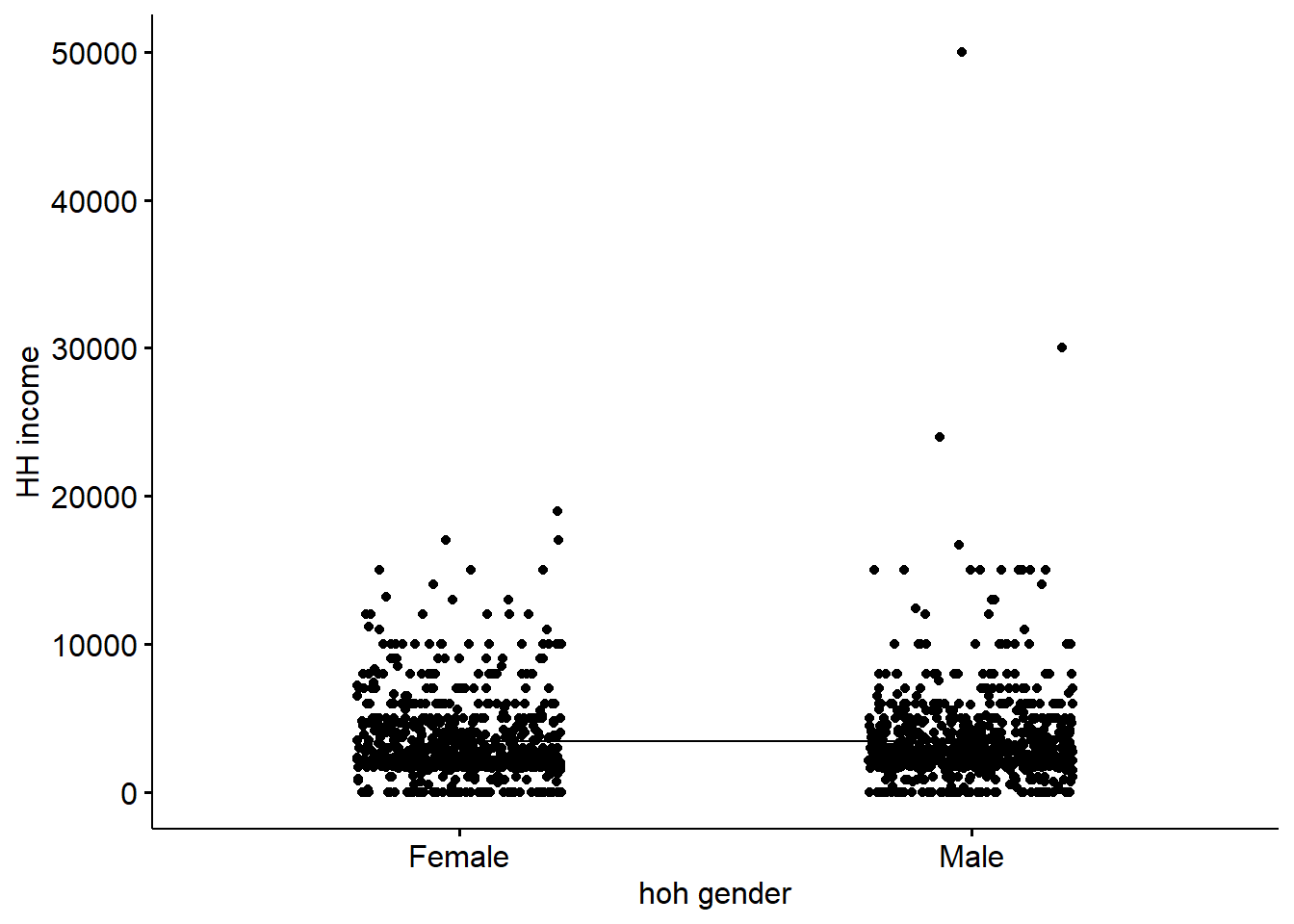

7.10.3 chi-squares

Pearson`s chi-squared test. Chi-squared test is a statistical hypothesis test, based on comparing expected and observed frequencies of 2-way distribution (2-way table).

There are three types of tests (hypothesis) that could be tested with chi-squared: independence of variables, homogenity of distribution of the characteristic across “stratas” and goodness of fit (whether the actual distribution is different from the hypothetical one). Two former versions use the same calculation.

Chi-squared test is a non-parametric test. It is used with nominal to nominal (nominal to ordinal) scales. For running chi-squared test, each cell of the crosstab should contain at least 5 observations.

Note, that chi-squared test indicates significance of differences in values on a table level. Thus, it is impossible to track significance in differences for particular options.

(For example, it is possible to say that satisfaction with public transport and living in urban / rural areas are connected. However, we can conclude from the test itself, that “satisfied” and “dissatisfied” options differ, while “indifferent” does not. By the way, it is possible to come up with this conclusion while interpreting a corresponding crosstab. Also, chi-squared test can tell nothing about the strength and the direction of a liaison between variables).

7.10.3.1 Chi-squared test for independence

The test for weighted data is being run with the survey library

library(survey)
library(dplyr)
library(weights)

The use of the survey package functions requires specifying survey design object (which reslects sampling approach).

main_dataset <- read.csv("inputs/UKR2007_MSNA20_HH_dataset_main_rcop.csv", na.strings = "", stringsAsFactors = F)

svy_design <- svydesign(data=main_dataset, 
                        id = ~1, 
                        strata = main_dataset$strata, 
                        probs = NULL,
                        weights = main_dataset$stratum.weight)

Specifying function for getting chi-squared outputs.

Hereby test Chi^2 test of independence is used. So, the test is performed to find out if strata variable and target variable are independent, H0 - the distribution of target variable values is equal across all stratas H1 - strata and target var are not independent, so distribution varies across stratas.

Apart from getting test statistic and p value, we would like to detect manually what are the biggest and the smallest values across groups/stratas (in case if the difference is significant and it makes sense to do it).

Hereby test Chi^2 test of independence is used. So, the test is performed to find out if strata variable and target variable are independent, H0 - the distribution of target var. values is equal across all stratas H1 - strata and target var are not independent, so distribution varies across stratas.

Within the Survey package, the suggested function uses Scott & Rao adjustment for complex survey design

#####Simple single call of the test.

Let’s say that the research aim is to understand whether the main water source is dependent on the area where HH lives (strata variable).

Thus, in our case: H0 - the distribution of water source is equal across stratas and these variables are independent H1 - the distribution of water source differs by strata and these variables are not independent.

Running the chi-squared test:

(Survey version - requires a survey design object)

svychisq(~ f11_dinking_water_source + strata, design = svy_design, statistic = "Chisq")

## 
##  Pearson's X^2: Rao & Scott adjustment
## 
## data:  svychisq(~f11_dinking_water_source + strata, design = svy_design,     statistic = "Chisq")
## X-squared = 244.62, df = 21, p-value < 2.2e-16

The current output presents the result of Pearson’s chi-squared test (Rao & Scott adjustment accounts for weighted data) [https://www.researchgate.net/publication/38360147_On_Simple_Adjustments_to_Chi-Square_Tests_with_Sample_Survey_Data].

The output consist of three parameters: 1. X-squared - observed value of chi-squared parameter, 2. df - “degrees of freedom” or number of independent categories in data -1 Having only these two elements it is possible to see, if with the current number of df, the value of chi-squared parameter is greater than the critical value for the chosen level of probability, using (tables of chi-squared critical values) [https://www.itl.nist.gov/div898/handbook/eda/section3/eda3674.htm] Fortunately, R provides us with the third parameter, which allows us to skip this step. 3. p-value - stands for the probability of getting value of the chi-squared parameter greater or equal to the given one assuming that H0 is true. If p-value < 0.05 (for 95% confidence level, or 0.01 for 99%), the H0 can be rejected.

In the current example, as p-value is very low, H0 can be rejected, and hence, strata variable and drinking water source are not independent.

(Weights package - can work with the dataframe directly, without the survey design object)

wtd.chi.sq(var1 = main_dataset$f11_dinking_water_source, var2 = main_dataset$strata, weight = main_dataset$stratum.weight)

##        Chisq           df      p.value 
## 2.446205e+02 2.100000e+01 4.928158e-40

Specifying the function for crosstabs with chi-squared tests for independence.

#####Functions to have test results along with crosstabs

The function with survey design object.

The function also helps to find out smallest and the largest values per row

chi2_ind_extr <- function(x, y, design){
  my_var <- y

# running Pearson's chi-squared test
  s_chi <- svychisq(as.formula(paste0("~", x,"+", y)), design, statistic = "Chisq")
  
  # extracting basic parameters
  wmy_t <- as.data.frame(s_chi$observed)
  wmy_t$p <- s_chi$p.value
  wmy_t$chi_adj <- s_chi$statistic
  wmy_t$df <- s_chi$parameter
  #indicating significance
  wmy_t$independence <- ifelse(wmy_t$p < 0.05, "h1", "h0")
  colnames(wmy_t)[1:2] <- c("var_x", "var_y")
  wmy_t_w <- spread(wmy_t, var_y, Freq)
  wmy_t_w[,1] <- paste0(x, " ", wmy_t_w[,1])
  colnames(wmy_t_w)[1] <- "variable"
  # getting percent from weighted frequencies
  cols_no_prop <- c("variable", "p", "independence", "max", "min", "chi_adj", "df")
  wmy_t_w[, !colnames(wmy_t_w) %in% cols_no_prop] <- lapply(wmy_t_w[, !colnames(wmy_t_w) %in% cols_no_prop], function(x){x/sum(x, na.rm = T)})
  # indicating extremum values
  cols_to_compare <- colnames(wmy_t_w)[!colnames(wmy_t_w) %in% c("p", "chi_adj", "df", "independence", "min", "max", "variable")]
  wmy_t_w$max <- ifelse(wmy_t_w$independence == "h1", cols_to_compare[apply(wmy_t_w, 1, which.max)], 0)
  
  wmy_t_w$min <- ifelse(wmy_t_w$independence == "h1", cols_to_compare[apply(wmy_t_w, 1, which.min)], 0)
  
  #adding Overall value to the table
  ovl_tab <- as.data.frame(prop.table(svytable(as.formula(paste0("~",x)), design)))
  colnames(ovl_tab) <- c("options", "overall")
  wmy_t_w <- wmy_t_w %>% bind_cols(ovl_tab)
  return(wmy_t_w)
}

The use with a single-choice question

chi2_ind_extr("f11_dinking_water_source", "strata", svy_design)

##                                                                                 variable
## 1                      f11_dinking_water_source bottled_water_water_purchased_in_bottles
## 2 f11_dinking_water_source drinking_water_from_water_kiosk_booth_with_water_for_bottling
## 3                                                 f11_dinking_water_source other_specify
## 4                                                 f11_dinking_water_source personal_well
## 5                        f11_dinking_water_source public_well_or_boreholes_shared_access
## 6                   f11_dinking_water_source tap_drinking_water_centralized_water_supply
## 7                                         f11_dinking_water_source technical_piped_water
## 8                        f11_dinking_water_source trucked_in_water_truck_with_a_tank_etc
##              p  chi_adj df independence 20km_rural 20km_urban   5km_rural
## 1 9.386389e-50 244.6205 21           h1 0.02457002 0.07673267 0.034825871
## 2 9.386389e-50 244.6205 21           h1 0.19901720 0.29950495 0.131840796
## 3 9.386389e-50 244.6205 21           h1 0.01228501 0.00000000 0.007462687
## 4 9.386389e-50 244.6205 21           h1 0.32432432 0.09653465 0.482587065
## 5 9.386389e-50 244.6205 21           h1 0.15724816 0.05445545 0.151741294
## 6 9.386389e-50 244.6205 21           h1 0.22358722 0.43316832 0.144278607
## 7 9.386389e-50 244.6205 21           h1 0.00000000 0.00000000 0.000000000
## 8 9.386389e-50 244.6205 21           h1 0.05896806 0.03960396 0.047263682
##     5km_urban       max        min
## 1 0.032178218 5km_rural 20km_urban
## 2 0.274752475 5km_rural 20km_urban
## 3 0.007425743 5km_rural       <NA>
## 4 0.121287129 5km_rural 20km_urban
## 5 0.099009901 5km_rural 20km_urban
## 6 0.383663366 5km_rural 20km_urban
## 7 0.004950495 5km_rural       <NA>
## 8 0.076732673 5km_rural 20km_urban
##                                                         options     overall
## 1                      bottled_water_water_purchased_in_bottles 0.049170548
## 2 drinking_water_from_water_kiosk_booth_with_water_for_bottling 0.263132750
## 3                                                 other_specify 0.005188695
## 4                                                 personal_well 0.167758525
## 5                        public_well_or_boreholes_shared_access 0.093728457
## 6                   tap_drinking_water_centralized_water_supply 0.362248561
## 7                                         technical_piped_water 0.001836837
## 8                        trucked_in_water_truck_with_a_tank_etc 0.056935627

In the given output, p indicates chi-squared test p-value, chi_adj - value of chi-squared parameter, df - degrees of freedom, independence - indicates which hypothesis is accepted, h0 or h1. In the current function, H1 is accepted if p < 0.05. In case H0 is rejected and H1 accepted, in min and max columns minimum and maximum y variable categories are given.

The use with a multiple-choice question.

The test would not work if any of dummies consists from zeros only, it need to be checked in advance, thus, let’s filter such variables out from the vector of variable names

Getting full range of dummies from the question

names <- names(main_dataset)
f12 <- names[grepl("f12_drinking_water_treat.", names)]

Defining a function which would remove zero-sum variables for us

if the absence of empty cells for each strata is needed, per_cell = T

non_zero_for_test <- function(var, strata, dataset, per_cell = F){
  sum <- as.data.frame(sapply(dataset[, names(dataset) %in% var], sum))
  sum <- cbind(rownames(sum), sum)
  filtered <- sum[sum[,2] > 0,1]
  tab <- as.data.frame(sapply(dataset[,names(dataset) %in% filtered], table, dataset[, strata]))
  ntab <- names(tab)
  #if the absence of empty cells for each strata is needed, per_cell = T
  tab <- tab[, which(colnames(tab) %in% ntab)]
  zeros <- apply(apply(tab, 2, function(x) x==0), 2, any)
  zeros <- zeros[zeros == F]
  zeros <- as.data.frame(zeros)
  zeros <- cbind(rownames(zeros), zeros)
  zeros_lab <- as.vector(unlist(strsplit(zeros[,1], split = ".Freq")))
  result <- c()
  if(per_cell == T){
    result <- zeros_lab
  } else {
    result <- ntab
  }
  message(paste0(abs(length(var) - length(result)), " variables were removed because of containing zeros in stratas"))
  
  return(result)
}

Using the test with multiple choice question.

nz_f12 <- non_zero_for_test(f12, "strata", main_dataset, per_cell = F)

## 2 variables were removed because of containing zeros in stratas

f12_sig <- lapply(nz_f12, chi2_ind_extr, y = "strata", design = svy_design)

f12_sig_df <- Reduce(rbind, f12_sig)

#removing 0 ("not selected") options
f12_sig_df <- f12_sig_df %>% filter(options == 1)
f12_sig_df

##                                                                variable
## 1       f12_drinking_water_treat.cleaning_with_chemicals_chlorination 1
## 2                        f12_drinking_water_treat.water_precipitation 1
## 3         f12_drinking_water_treat.filtering_the_water_pitcher_filter 1
## 4 f12_drinking_water_treat.filtering_the_water_reverse_osmosis_filter 1
## 5                                    f12_drinking_water_treat.boiling 1
## 6                                f12_drinking_water_treat.percolation 1
## 7                              f12_drinking_water_treat.other_specify 1
## 8                      f12_drinking_water_treat.do_not_process_purify 1
##            p  chi_adj df independence  20km_rural  20km_urban   5km_rural
## 1 0.03100696 4.780006  3           h1 0.000000000 0.004950495 0.000000000
## 2 0.02775288 7.977278  3           h1 0.073710074 0.126237624 0.104477612
## 3 0.55635016 1.828231  3           h0 0.046683047 0.069306931 0.059701493
## 4 0.44029529 2.347539  3           h0 0.027027027 0.037128713 0.017412935
## 5 0.02724163 8.191084  3           h1 0.260442260 0.274752475 0.223880597
## 6 0.24801653 3.459406  3           h0 0.004914005 0.002475248 0.007462687
## 7 0.28029092 2.860754  3           h0 0.004914005 0.002475248 0.000000000
## 8 0.01762880 9.011919  3           h1 0.624078624 0.551980198 0.674129353
##    5km_urban       max        min options     overall
## 1 0.00000000 5km_rural       <NA>       1 0.002000313
## 2 0.14108911 5km_rural 20km_urban       1 0.122036605
## 3 0.06930693         0          0       1 0.065108190
## 4 0.04207921         0          0       1 0.036036995
## 5 0.20792079 5km_rural 20km_urban       1 0.244239386
## 6 0.00000000         0          0       1 0.002279393
## 7 0.00000000         0          0       1 0.001769625
## 8 0.60643564 5km_rural 20km_urban       1 0.591818943

The function without the survey design object

chi2_ind_wtd <- function(x, y, weight, dataset){
  i <- 1
  table_new <- data.frame()
  for (i in 1:length(x)) {
  ni <- x[i]
  ti <- dataset %>% 
    filter(!is.na(!!sym(y))) %>%
    group_by(!!sym(y), !!sym(ni)) %>% 
    filter(!is.na(!!sym(ni))) %>%
    summarise(wtn = sum(!!sym(weight)), n = n()) %>%
    mutate(prop = wtn/sum(wtn), varnam = ni)
  names(ti) <- c("var_ind", "var_dep_val", "wtn", "n",  "prop", "dep_var_nam")
  ti <- ti %>% ungroup() %>% mutate(base = sum(c_across(n)))
  chi_test  <- wtd.chi.sq(var1 = dataset[, paste0(y)], var2 = dataset[, paste0(ni)], weight = dataset[, paste0(weight)])
  ti$chisq <- chi_test[1]
  ti$df <- chi_test[2]
  ti$p <- chi_test[3]
  ti$hypo <- ifelse(ti$p < 0.05, "h1", "h0")
  table_new <- rbind(table_new, ti)
}
table_cl_new_1 <- table_new %>% 
  #filter(var_dep_val != "0") %>% 
  filter(!is.na(var_dep_val))
#mutate(var_id = paste0(dep_var_nam, ".", var_dep_val))
table_cl_new_1 <- table_cl_new_1[, -c(3, 4)]

table_sprd <- tidyr::spread(table_cl_new_1, var_ind, prop) %>%
  arrange(dep_var_nam)
return(table_sprd)
}

The use with the single choice question

chi2_ind_wtd(x = "f11_dinking_water_source", y = "strata",
             weight = "stratum.weight", main_dataset)

## `summarise()` has grouped output by 'strata'. You can
## override using the `.groups` argument.

## # A tibble: 8 × 11
##   var_dep_val          dep_var_nam  base chisq    df        p hypo  `20km_rural`
##   <chr>                <chr>       <int> <dbl> <dbl>    <dbl> <chr>        <dbl>
## 1 bottled_water_water… f11_dinkin…  1617  245.    21 4.93e-40 h1          0.0246
## 2 drinking_water_from… f11_dinkin…  1617  245.    21 4.93e-40 h1          0.199 
## 3 other_specify        f11_dinkin…  1617  245.    21 4.93e-40 h1          0.0123
## 4 personal_well        f11_dinkin…  1617  245.    21 4.93e-40 h1          0.324 
## 5 public_well_or_bore… f11_dinkin…  1617  245.    21 4.93e-40 h1          0.157 
## 6 tap_drinking_water_… f11_dinkin…  1617  245.    21 4.93e-40 h1          0.224 
## 7 technical_piped_wat… f11_dinkin…  1617  245.    21 4.93e-40 h1         NA     
## 8 trucked_in_water_tr… f11_dinkin…  1617  245.    21 4.93e-40 h1          0.0590
## # … with 3 more variables: `20km_urban` <dbl>, `5km_rural` <dbl>,
## #   `5km_urban` <dbl>

The use with multiple choice questions

names <- names(main_dataset)

f12_names <- names[grepl("f12_drinking_water_treat.", names)]

f12_sig2 <- lapply(f12_names, chi2_ind_wtd, y = "strata", weight = "stratum.weight", main_dataset)

f12_tab_df <- Reduce(rbind, f12_sig2)
f12_tab_df

## # A tibble: 18 × 11
##    var_dep_val dep_var_nam            base chisq    df      p hypo  `20km_rural`
##          <int> <chr>                 <int> <dbl> <dbl>  <dbl> <chr>        <dbl>
##  1           0 f12_drinking_water_t…  1617  4.78     3 0.189  h0         1      
##  2           1 f12_drinking_water_t…  1617  4.78     3 0.189  h0        NA      
##  3           0 f12_drinking_water_t…  1617  7.98     3 0.0465 h1         0.926  
##  4           1 f12_drinking_water_t…  1617  7.98     3 0.0465 h1         0.0737 
##  5           0 f12_drinking_water_t…  1617  1.83     3 0.609  h0         0.953  
##  6           1 f12_drinking_water_t…  1617  1.83     3 0.609  h0         0.0467 
##  7           0 f12_drinking_water_t…  1617  2.35     3 0.503  h0         0.973  
##  8           1 f12_drinking_water_t…  1617  2.35     3 0.503  h0         0.0270 
##  9           0 f12_drinking_water_t…  1617  8.19     3 0.0422 h1         0.740  
## 10           1 f12_drinking_water_t…  1617  8.19     3 0.0422 h1         0.260  
## 11           0 f12_drinking_water_t…  1617  3.46     3 0.326  h0         0.995  
## 12           1 f12_drinking_water_t…  1617  3.46     3 0.326  h0         0.00491
## 13           0 f12_drinking_water_t…  1617  2.86     3 0.414  h0         0.995  
## 14           1 f12_drinking_water_t…  1617  2.86     3 0.414  h0         0.00491
## 15           0 f12_drinking_water_t…  1617  0        0 1      h0         1      
## 16           0 f12_drinking_water_t…  1617  0        0 1      h0         1      
## 17           0 f12_drinking_water_t…  1617  9.01     3 0.0291 h1         0.376  
## 18           1 f12_drinking_water_t…  1617  9.01     3 0.0291 h1         0.624  
## # … with 3 more variables: `20km_urban` <dbl>, `5km_rural` <dbl>,
## #   `5km_urban` <dbl>

7.10.4 Chi-squared Goodness of Fit test

Goodness of test chi-squared test is used to compare the observed distribution with the hypothetical one,

For instance, we would like to test the hypothesis, that 90% of HHs had soap in their HHs at the moment of the survey.

main_dataset <- main_dataset %>% mutate(soap = case_when(
 p16_soap_household == "dont_know_refuse_to_answer" ~ "NA",
 p16_soap_household == "no" ~ "no",
 p16_soap_household == "yes_soap_is_not_shown" ~ "yes",
 p16_soap_household == "yes_soap_is_shown" ~ "yes"
))
soap_prob <- as.data.frame(prop.table(table(main_dataset$soap)))
soap_prob <- soap_prob[, 2]
# please, note that this is a function call with unweighted data!
chisq.test(soap_prob, p = c(0, 0.1, 0.9))

## Warning in chisq.test(soap_prob, p = c(0, 0.1, 0.9)): Chi-squared approximation
## may be incorrect

## 
##  Chi-squared test for given probabilities
## 
## data:  soap_prob
## X-squared = Inf, df = 2, p-value < 2.2e-16

As p value is lower than the chosen confidence level, hypothesis of equality of the current distribution to hypothetical 90% / 10% of soap-owners can be rejected.

Defining a function for checking the distribution within a particular group, against the “hypothetical” overall sample.

For the overall sample we would need a variable which has the same value across all observations (e.g. informed consent == yes etc.)

chi2_GoF <- function(name, stratum_hyp, stratum_2, value_stratum_hyp, value_stratum_2, data, weights){
  i <- 1
  table_1 <- data.frame()
  for (i in 1:length(name)) {
    ni <- name[i]
    ti <- data %>% 
      group_by(!!sym(ni)) %>% filter(!!sym(stratum_hyp) == paste0(value_stratum_hyp)) %>%
      filter(!is.na(!!sym(ni))) %>%
      summarise(wtn = sum(!!sym(weights)), n = n()) %>%
      mutate(prop = wtn/sum(wtn), base = sum(wtn), cnt = sum(n))%>%
      mutate(varnam = ni)
    names(ti) <- c("var", "wtn", "n", "prop", "base_w", "count", "nam")
    table_1 <- rbind(table_1, ti)
  }
  table_cl_1 <- table_1 %>% filter(!is.na(var)) %>%
    mutate(var_id = paste0(nam, ".", var))
  i <- 1
  table_2 <- data.frame()
  for (i in 1:length(name)) {
    ni <- name[i]
    ti <- data %>% 
      group_by(!!sym(ni)) %>% filter(!!sym(stratum_2) == paste0(value_stratum_2)) %>%
      filter(!is.na(!!sym(ni))) %>%
      summarise(wtn = sum(!!sym(weights)), n = n()) %>%
      mutate(prop = wtn/sum(wtn), base = sum(wtn), cnt = sum(n))%>%
      mutate(varnam = ni)
    names(ti) <- c("var", "wtn", "n", "prop", "base_w", "count", "nam")
    table_2 <- rbind(table_2, ti)
  }
  
  table_cl_2 <- table_2 %>% filter(!is.na(var)) %>%
    mutate(var_id = paste0(nam, ".", var))
  table_cl_compare <- merge(table_cl_1, table_cl_2, by = "var_id", all = T)
  names(table_cl_compare) <- c("var.id", "var.hyp", "wtn.hyp", "n.hyp", "prop.hyp", "base.hyp", "base_nw.hyp","nam.hyp", "var.2", "wtn.2", "n.2", "prop.2", "base.2", "base_nw.2", "nam.2")
  
  #Dealing with NA issues
  table_cl_compare$nam.hyp[is.na(table_cl_compare$nam.hyp)] <- table_cl_compare$nam.2[is.na(table_cl_compare$nam.hyp)]
  
  table_cl_compare$nam.2[is.na(table_cl_compare$nam.2)] <- table_cl_compare$nam.hyp[is.na(table_cl_compare$nam.2)]
  
  table_cl_compare$to_split <- table_cl_compare$nam.hyp
  
  table_cl_compare <- separate(table_cl_compare, col = to_split, into = c("indctr", "item"), sep ="\\.")
  
  table_cl_compare <- table_cl_compare %>% group_by(indctr) %>% fill(base_nw.hyp, .direction  = "down") %>% fill(base_nw.hyp, .direction  = "up") %>% ungroup()
  table_cl_compare <- table_cl_compare %>% group_by(indctr) %>% fill(base.hyp, .direction  = "down") %>% fill(base.hyp, .direction  = "up") %>% ungroup()
  table_cl_compare <- table_cl_compare %>% group_by(indctr) %>% fill(base_nw.2, .direction  = "down") %>% fill(base_nw.2, .direction  = "up") %>% ungroup()
  table_cl_compare <- table_cl_compare %>% group_by(indctr) %>% fill(base.2) %>% fill(base_nw.hyp, .direction  = "down") %>% fill(base.2, .direction  = "up") %>% ungroup()
  
  table_cl_compare$prop.hyp[is.na(table_cl_compare$prop.hyp)] <- 0
  table_cl_compare$prop.2[is.na(table_cl_compare$prop.2)] <- 0
  
  table_cl_compare$wtn.hyp[is.na(table_cl_compare$wtn.hyp)] <- 0
  table_cl_compare$wtn.2[is.na(table_cl_compare$wtn.2)] <- 0
  
  table_cl_compare$chi2 <- chisq.test(table_cl_compare$wtn.2, p = table_cl_compare$prop.hyp)$statistic
  table_cl_compare$p <- chisq.test(table_cl_compare$wtn.2, p = table_cl_compare$prop.hyp)$p.value
  table_cl_compare$df <- chisq.test(table_cl_compare$wtn.2, p = table_cl_compare$prop.hyp)$df
  
  table_cl_compare$H0 <- ifelse(table_cl_compare$p <= 0.05, "H1 - different", "H0 - same")
  return(table_cl_compare)
}

Using the function with a single choice question

chi2_GoF(name = "f11_dinking_water_source", stratum_hyp = "a1_informed_consent", stratum_2 = "strata", value_stratum_hyp = "yes", value_stratum_2 = "5km_rural", data = main_dataset, weights = "stratum.weight")

## Warning: Expected 2 pieces. Missing pieces filled with `NA` in 8 rows [1, 2, 3,
## 4, 5, 6, 7, 8].

## Warning in chisq.test(table_cl_compare$wtn.2, p = table_cl_compare$prop.hyp):
## Chi-squared approximation may be incorrect

## Warning in chisq.test(table_cl_compare$wtn.2, p = table_cl_compare$prop.hyp):
## Chi-squared approximation may be incorrect

## Warning in chisq.test(table_cl_compare$wtn.2, p = table_cl_compare$prop.hyp):
## Chi-squared approximation may be incorrect

## # A tibble: 8 × 20
##   var.id       var.hyp wtn.hyp n.hyp prop.hyp base.hyp base_nw.hyp nam.hyp var.2
##   <chr>        <chr>     <dbl> <int>    <dbl>    <dbl>       <int> <chr>   <chr>
## 1 f11_dinking… bottle…   79.5     68  0.0492     1617.        1617 f11_di… bott…
## 2 f11_dinking… drinki…  425.     366  0.263      1617.        1617 f11_di… drin…
## 3 f11_dinking… other_…    8.39    11  0.00519    1617.        1617 f11_di… othe…
## 4 f11_dinking… person…  271.     414  0.168      1617.        1617 f11_di… pers…
## 5 f11_dinking… public…  152.     187  0.0937     1617.        1617 f11_di… publ…
## 6 f11_dinking… tap_dr…  586.     479  0.362      1617.        1617 f11_di… tap_…
## 7 f11_dinking… techni…    2.97     2  0.00184    1617.        1617 f11_di… <NA> 
## 8 f11_dinking… trucke…   92.1     90  0.0569     1617.        1617 f11_di… truc…
## # … with 11 more variables: wtn.2 <dbl>, n.2 <int>, prop.2 <dbl>, base.2 <dbl>,
## #   base_nw.2 <int>, nam.2 <chr>, indctr <chr>, item <chr>, chi2 <dbl>,
## #   p <dbl>, H0 <chr>

Using the function with the multiple responce set

names <- names(main_dataset)

f12_names <- names[grepl("f12_drinking_water_treat.", names)]

#removing empty variables from the MR set
nz_f12 <- non_zero_for_test(f12_names, "strata", main_dataset, per_cell = F)

## 2 variables were removed because of containing zeros in stratas

table(main_dataset[, nz_f12[4]], main_dataset[, "strata"])

##    
##     20km_rural 20km_urban 5km_rural 5km_urban
##   0        396        389       395       387
##   1         11         15         7        17

f12_sig2 <- lapply(nz_f12, chi2_GoF, stratum_hyp = "a1_informed_consent", stratum_2 = "strata", value_stratum_hyp = "yes", value_stratum_2 = "5km_rural", data = main_dataset, weights = "stratum.weight")

f12_sig2_df <- Reduce(rbind, f12_sig2)
f12_sig2_df

## # A tibble: 16 × 20
##    var.id      var.hyp wtn.hyp n.hyp prop.hyp base.hyp base_nw.hyp nam.hyp var.2
##    <chr>         <int>   <dbl> <int>    <dbl>    <dbl>       <int> <chr>   <int>
##  1 f12_drinki…       0 1614.    1615  0.998      1617.        1617 f12_dr…     0
##  2 f12_drinki…       1    3.23     2  0.00200    1617.        1617 f12_dr…    NA
##  3 f12_drinki…       0 1420.    1437  0.878      1617.        1617 f12_dr…     0
##  4 f12_drinki…       1  197.     180  0.122      1617.        1617 f12_dr…     1
##  5 f12_drinki…       0 1512.    1518  0.935      1617.        1617 f12_dr…     0
##  6 f12_drinki…       1  105.      99  0.0651     1617.        1617 f12_dr…     1
##  7 f12_drinki…       0 1559.    1567  0.964      1617.        1617 f12_dr…     0
##  8 f12_drinki…       1   58.3     50  0.0360     1617.        1617 f12_dr…     1
##  9 f12_drinki…       0 1222.    1226  0.756      1617.        1617 f12_dr…     0
## 10 f12_drinki…       1  395.     391  0.244      1617.        1617 f12_dr…     1
## 11 f12_drinki…       0 1613.    1611  0.998      1617.        1617 f12_dr…     0
## 12 f12_drinki…       1    3.69     6  0.00228    1617.        1617 f12_dr…     1
## 13 f12_drinki…       0 1614.    1614  0.998      1617.        1617 f12_dr…     0
## 14 f12_drinki…       1    2.86     3  0.00177    1617.        1617 f12_dr…    NA
## 15 f12_drinki…       0  660.     624  0.408      1617.        1617 f12_dr…     0
## 16 f12_drinki…       1  957.     993  0.592      1617.        1617 f12_dr…     1
## # … with 11 more variables: wtn.2 <dbl>, n.2 <int>, prop.2 <dbl>, base.2 <dbl>,
## #   base_nw.2 <int>, nam.2 <chr>, indctr <chr>, item <chr>, chi2 <dbl>,
## #   p <dbl>, H0 <chr>

7.10.5 Proportion tests (z-test)

Test for equality of proportions for independent samples. To compare column proportions for independent samples, two tailed z-test of proportions could be used.

Main assumptions of use of this test are:

normally distributed data
sample size > 30 and n at each point >= 5 (!Thus, for the variables were there are few observations, approximation could be incorrect!) The detailed explanation of this statistic and its use in R could be found here: http://www.sthda.com/english/wiki/two-proportions-z-test-in-r

As in our datasets weighting is used, in the current test, we use weighted proportions and weighted counts for calculating test statistics.

zprop_compare_weighted <- function(data_old, data_new, stratum, value_stratum, name, weights, strict = F){
  names_new <- names(data_new)
  not_in_new <- names_new[which(!(name %in% names_new))]
i <- 1
table_old <- data.frame()
for (i in 1:length(name)) {
  ni <- name[i]
  ti <- data_old %>% 
    group_by(!!sym(ni)) %>% filter(!!sym(stratum) == paste0(value_stratum)) %>%
    filter(!is.na(!!sym(ni))) %>%
    filter(!!sym(ni) != 'refuse') %>%
    dplyr::summarize(wtn = sum(!!sym(weights)), n = n()) %>%
    mutate(prop = wtn/sum(wtn), base = sum(wtn), cnt = sum(n))%>%
    mutate(varnam = ni)
  names(ti) <- c("var", "wtn", "n", "prop", "base_w", "count", "nam")
  table_old <- rbind(table_old, ti)
}
table_cl_old <- table_old %>% filter(var != "0") %>% filter(!is.na(var)) %>%
  mutate(var_id = paste0(nam, ".", var))
i <- 1
table_new <- data.frame()
for (i in 1:length(name)) {
  ni <- name[i]
  ti <- data_new %>% 
    group_by(!!sym(ni)) %>% filter(!!sym(stratum) == paste0(value_stratum)) %>%
    filter(!is.na(!!sym(ni))) %>%
    filter(!!sym(ni) != 'refuse') %>%
    dplyr::summarize(wtn = sum(!!sym(weights)), n = n()) %>%
    mutate(prop = wtn/sum(wtn), base = sum(wtn), cnt = sum(n))%>%
    mutate(varnam = ni)
  names(ti) <- c("var", "wtn", "n", "prop", "base_w", "count", "nam")
  table_new <- rbind(table_new, ti)
}
table_cl_new <- table_new %>% filter(var != "0") %>% filter(!is.na(var)) %>%
  mutate(var_id = paste0(nam, ".", var))
table_cl_compare <- merge(table_cl_old, table_cl_new, by = "var_id", all = T)
names(table_cl_compare) <- c("var.id", "var.old", "wtn.old", "n.old", "prop.old", "base.old", "base_nw.old","nam.old", "var.new", "wtn.new", "n.new", "prop.new", "base.new", "base_nw.new", "nam.new")

#Dealing with NA issues

  table_cl_compare$nam.old[is.na(table_cl_compare$nam.old)] <- table_cl_compare$nam.new[is.na(table_cl_compare$nam.old)]
  
    table_cl_compare$nam.new[is.na(table_cl_compare$nam.new)] <- table_cl_compare$nam.old[is.na(table_cl_compare$nam.new)]

table_cl_compare$to_split <- table_cl_compare$nam.old
  
table_cl_compare <- separate(table_cl_compare, col = to_split, into = c("indctr", "item"), sep ="\\.")

  table_cl_compare <- table_cl_compare %>% group_by(indctr) %>% fill(base_nw.old, .direction  = "down") %>% fill(base_nw.old, .direction  = "up") %>% ungroup()
  table_cl_compare <- table_cl_compare %>% group_by(indctr) %>% fill(base.old, .direction  = "down") %>% fill(base.old, .direction  = "up") %>% ungroup()
  table_cl_compare <- table_cl_compare %>% group_by(indctr) %>% fill(base_nw.new, .direction  = "down") %>% fill(base_nw.new, .direction  = "up") %>% ungroup()
  table_cl_compare <- table_cl_compare %>% group_by(indctr) %>% fill(base.new) %>% fill(base_nw.old, .direction  = "down") %>% fill(base.new, .direction  = "up") %>% ungroup()


table_cl_compare$prop.old[is.na(table_cl_compare$prop.old)] <- 0
table_cl_compare$prop.new[is.na(table_cl_compare$prop.new)] <- 0

table_cl_compare$wtn.old[is.na(table_cl_compare$wtn.old)] <- 0
table_cl_compare$wtn.new[is.na(table_cl_compare$wtn.new)] <- 0

for (i in 1:nrow(table_cl_compare)){
pt <- prop.test(x = c(table_cl_compare$wtn.old[i], table_cl_compare$wtn.new[i]), n = c(table_cl_compare$base.old[i], table_cl_compare$base.new[i]))
table_cl_compare$prp_tst_p[i] <- pt$p.value
}
table_cl_compare$sig <- ifelse(table_cl_compare$prp_tst_p < 0.05, "Significant diff.", "Not significant")
table_cl_compare$stratum <- paste0(value_stratum)


table_cl_compare_final <- table_cl_compare %>% 
  filter(case_when(strict == T ~ (prop.old*n.new >= 10 & prop.old*n.old >=10),
                   strict == F ~ (base_nw.old >= 30 & base_nw.new >=30)))

table_cl_compare_final <- table_cl_compare_final %>% filter(!(nam.old %in% not_in_new))

if(nrow(table_cl_compare_final) < nrow(table_cl_compare)){
  ss_vars <- table_cl_compare$var.id[which(!(table_cl_compare$var.id %in% table_cl_compare_final$var.id))]
  warning(paste0("Too small sample size. Variables that were removed from the analysis", ss_vars))
}

return(table_cl_compare_final)
}

7.10.5.0.1 Applying the function

Z-tests can be used for wave to wave or round to round comparisons.

Assuming, there was staged data collection and at stage1 Luhansk oblast was assessed, while at stage2 Donetsk oblast was assessed (it is an artificial division, for correct comparison between wave), hence we have two different datasets for Donetska and Luhanska regions (UA14 and UA44 respectively) and the question is whether proportions of female-led households, living in each shelter type are the same.

Thus, H0 - proportions are the same, H1 - proportions are different.

ds_ua14 <- main_dataset |> filter(r1_current_oblast == "UA14")
ds_ua44 <- main_dataset |> filter(r1_current_oblast == "UA44")

Applying the function for single choices

data_old, data_new - dataset1 and dataset2;
stratum - independent variable (should be the same for both datasets), if there is no need for independent variable, variable that have same value across the entire dataset can be used (e.g. “informed consent”);
value_stratum - independent variable value, that should be used for crosstabulations (e.g. we would like to compare the proportions for certain settlement or household type);
name - dependent variable name;
weights - weighting variable;
strict - (TRUE/FALSE) specifies if the less strict restrictment to sample size (n>30) or more strict one (n at each point >= 5) should be applied. FALSE be default

library(dplyr)
# without independent variable
marital_prop_test <- zprop_compare_weighted(data_old = ds_ua14, data_new = ds_ua44, stratum = "a1_informed_consent", value_stratum = "yes", name = "b9_hohh_marital_status", weights = "stratum.weight")

marital_prop_test

## # A tibble: 6 × 20
##   var.id     var.old wtn.old n.old prop.old base.old base_nw.old nam.old var.new
##   <chr>      <chr>     <dbl> <int>    <dbl>    <dbl>       <int> <chr>   <chr>  
## 1 b9_hohh_m… divorc…   141.    127   0.116     1220.        1168 b9_hoh… divorc…
## 2 b9_hohh_m… married   538.    515   0.441     1220.        1168 b9_hoh… married
## 3 b9_hohh_m… separa…    33.3    32   0.0273    1220.        1168 b9_hoh… separa…
## 4 b9_hohh_m… single    113.     99   0.0924    1220.        1168 b9_hoh… single 
## 5 b9_hohh_m… unmarr…    61.6    65   0.0505    1220.        1168 b9_hoh… unmarr…
## 6 b9_hohh_m… widowed   333.    330   0.273     1220.        1168 b9_hoh… widowed
## # … with 11 more variables: wtn.new <dbl>, n.new <int>, prop.new <dbl>,
## #   base.new <dbl>, base_nw.new <int>, nam.new <chr>, indctr <chr>, item <chr>,
## #   prp_tst_p <dbl>, sig <chr>, stratum <chr>

# with an independent variable
house_type_married <- zprop_compare_weighted(data_old = ds_ua14, data_new = ds_ua44, stratum = "b9_hohh_marital_status", value_stratum = "married", name = "e2_home_type", weights = "stratum.weight")

Output numeric columns: - wtn.old - weighted counts for the first (old) data - n.old - unweighted counts for the first (old) data - prop.old - weighted proportion for the first (old) data - base.old - weighted base (total count) for the first (old) data - base_nw.old - unweighted base (total count) for the first (old) data - wtn.new - weighted counts for the second (new) data - n.new - unweighted counts for the second (new) data - prop.new - weighted proportion for for the second (new) data - base.new - weighted base (total count) for the second (new) data - base_nw.new - unweighted base (total count) for the second (new) data - prp_tst_p - p-value for proportions test - sig - indication if p<0.05

Applying the function for multiple choice questions

names <- names(ds_ua14)
ng5 <- names[grepl("b10_hohh_vulnerability", names)]

vulnerability_prop_test <- zprop_compare_weighted(data_old = ds_ua14, data_new = ds_ua44, stratum = "a1_informed_consent", value_stratum = "yes", name = ng5, weights = "stratum.weight")

vulnerability_prop_test

## # A tibble: 61 × 20
##    var.id    var.old wtn.old n.old prop.old base.old base_nw.old nam.old var.new
##    <chr>     <chr>     <dbl> <int>    <dbl>    <dbl>       <int> <chr>   <chr>  
##  1 b10_hohh… chroni…  75.3      68 0.0618      1220.        1168 b10_ho… chroni…
##  2 b10_hohh… chroni…   7.38      7 0.00605     1220.        1168 b10_ho… chroni…
##  3 b10_hohh… chroni…  16.4      24 0.0134      1220.        1168 b10_ho… chroni…
##  4 b10_hohh… chroni…   0.275     1 0.000225    1220.        1168 b10_ho… <NA>   
##  5 b10_hohh… chroni…  10.4      11 0.00855     1220.        1168 b10_ho… chroni…
##  6 b10_hohh… 1       505.      496 0.414       1220.        1168 b10_ho… 1      
##  7 b10_hohh… disabi…  24.8      24 0.0204      1220.        1168 b10_ho… disabi…
##  8 b10_hohh… disabi…  12.4      10 0.0102      1220.        1168 b10_ho… disabi…
##  9 b10_hohh… disabi…   4.99      4 0.00410     1220.        1168 b10_ho… <NA>   
## 10 b10_hohh… disabi…   2.03      3 0.00167     1220.        1168 b10_ho… <NA>   
## # … with 51 more rows, and 11 more variables: wtn.new <dbl>, n.new <int>,
## #   prop.new <dbl>, base.new <dbl>, base_nw.new <int>, nam.new <chr>,
## #   indctr <chr>, item <chr>, prp_tst_p <dbl>, sig <chr>, stratum <chr>